Advanced Documentation

version 2.1.0

First steps into automatic inking

Introduction

Important

While this guide uses the API approach, it provides a solid foundation for understanding the underlying process.

Archaeological drawing digitisation represents a crucial step in preserving and sharing our cultural heritage. While traditionally done by hand, modern computational methods can help streamline this process while maintaining the high standards required for archaeological documentation. This guide walks you through using the ink module, a specialised tool designed for converting pencil drawings of archaeological artefacts into publication-ready inked versions.

Setting Up Your Environment

Let’s begin by importing the necessary functions from the toolset:

from ink import process_folder, run_diagnostics

These two functions serve as the foundation of our processing pipeline. The run_diagnostics function helps us understand how our images will interact with the model, while process_folder handles the actual conversion process.

Think of run_diagnostics as our planning phase and process_folder as our execution phase.

Understanding the Diagnostic Process

Before processing an entire collection of drawings, we need to understand how our specific drawings will interact with the model.

First, let’s set up our working directory:

my_path = "Montale_example"

Now we can run our diagnostic analysis:

run_diagnostics(
    input_folder=my_path,           # Where your drawings are stored
    model_path="6h-MCG.pkl",        # The trained model file
    num_sample_images=1,            # How many test images to analyze
    contrast_values=[0.5, 0.75, 1, 1.5, 2, 3],  # Different contrast levels to test
)

Let’s understand each parameter in detail:

• input_folder: This is where your pencil drawings are stored. The function will randomly select images from this folder for analysis.
• model_path: Points to your trained model file. This model contains the learned patterns for converting pencil drawings to inked versions.
• num_sample_images: Controls how many images to analyse. For a small collection, 1-2 images might suffice, but for larger collections with varying drawing styles, you might want to test more.
• contrast_values: These values help us understand how different contrast levels affect the model’s output. Think of this like adjusting the pressure of your pen when inking - too light (low contrast) might lose details, while too heavy (high contrast) might create unwanted artefacts.

The diagnostic process creates a structured output that helps us understand how our images will be processed:

diagnostic/
├── contrast_analysis_{progressive_number}.png  # Shows how contrast affects results
├── patches_{progressive_number}.png            # Shows how images will be divided
└── summary_{progressive_number}.txt            # Contains detailed analysis

Let’s examine the patch division output (Figure 1):

Figure 1: This visualization shows how your image will be processed in smaller chunks.

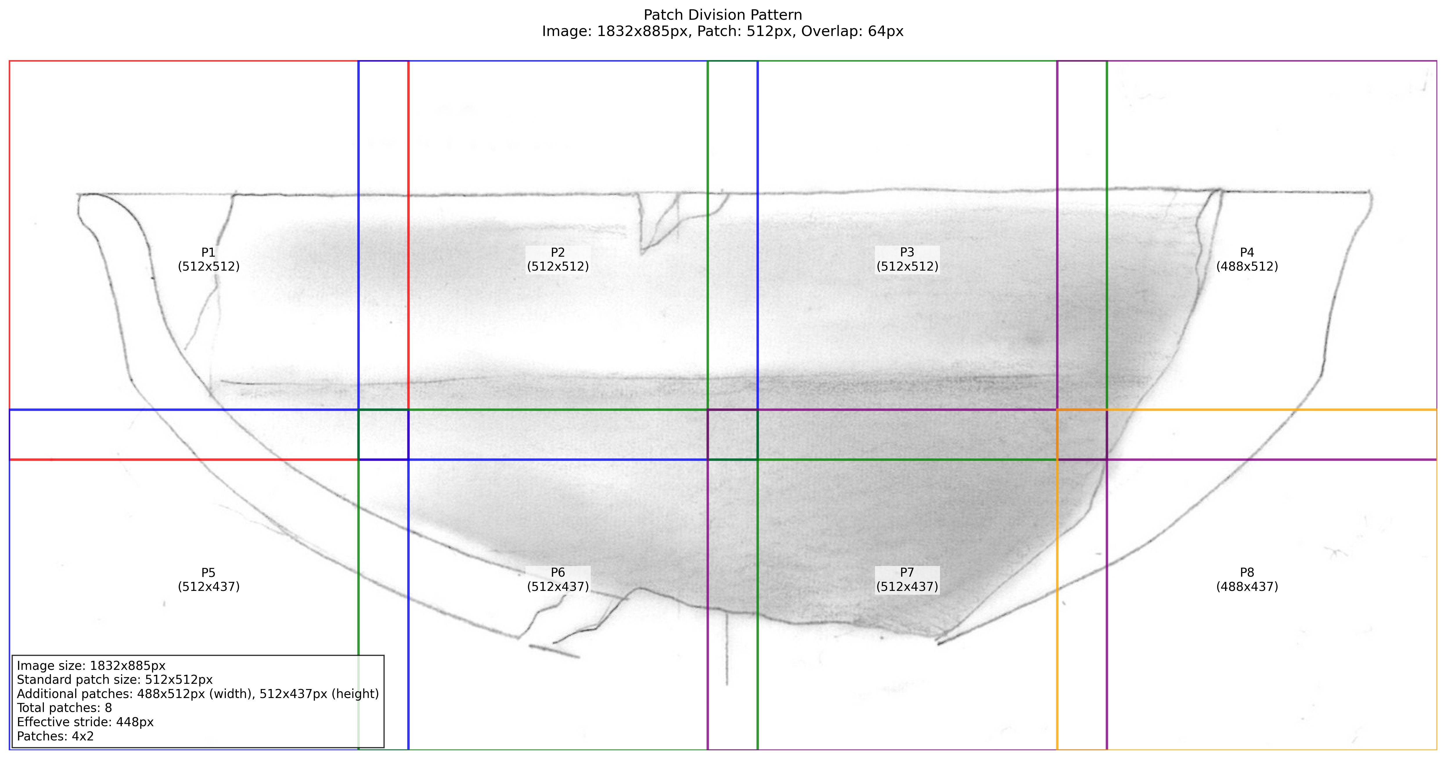
The patch division is crucial because it shows us how the model will break down larger images into manageable pieces. The overlap between patches helps prevent visible seams in the final output.

Next, let’s look at the contrast analysis (Figure 2):

Figure 2: This analysis shows how different contrast values affect the model’s output. Notice how extreme values can either lose detail (too low) or create artefacts (too high).

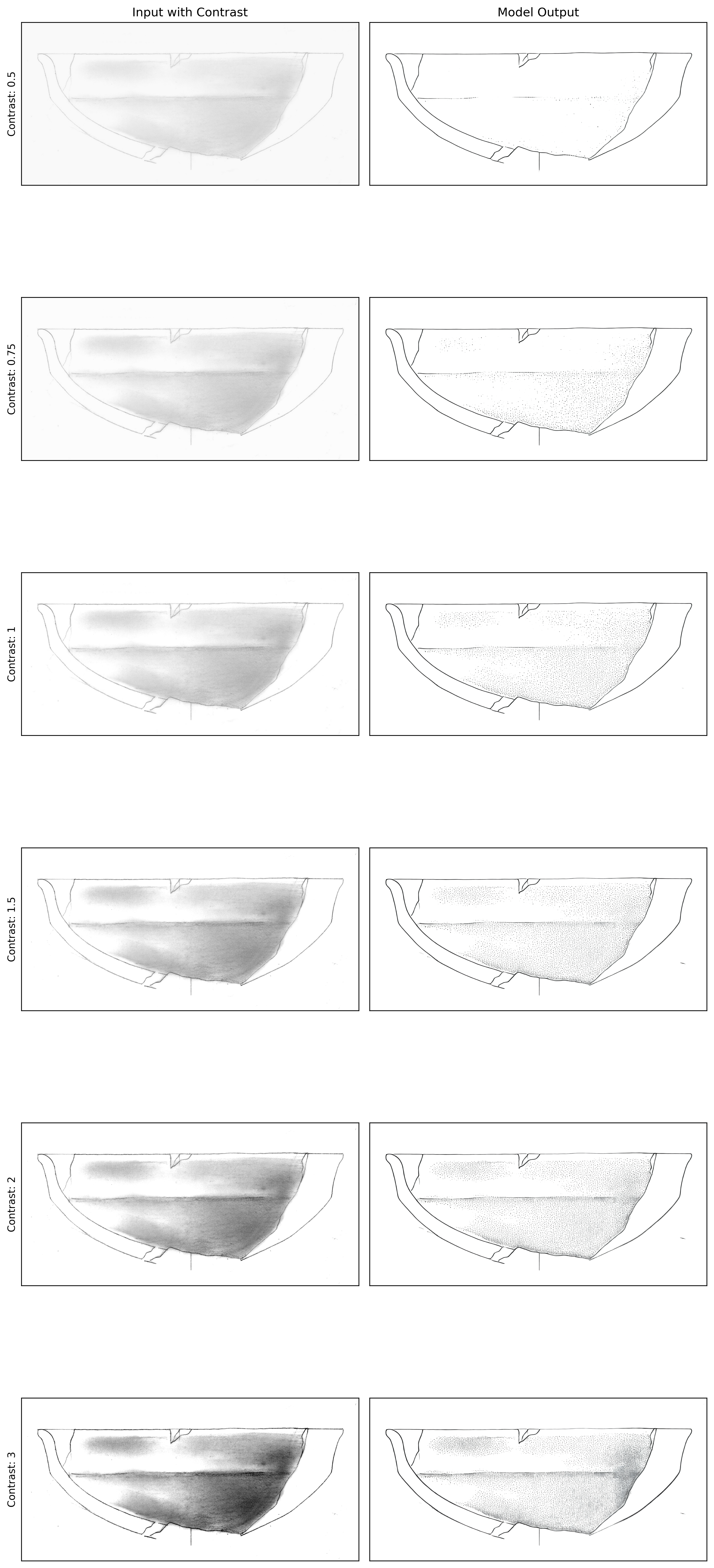
This visualization is particularly important because it helps us find the sweet spot for contrast enhancement. Looking at the results:

• A contrast value of 0.5 is too low, causing loss of fine details
• A contrast value of 3.0 is too high, introducing unwanted artefacts
• Values between 1.0 and 1.5 seem to produce the most balanced results

Processing Your Collection

After understanding how our images interact with the model through diagnostics, we can proceed with processing our entire collection:

process_folder(
    input_folder=my_path,
    model_path="6h-MCG.pkl",
    contrast_scale=1.25,            # Chosen based on diagnostic results
    output_dir="Montale_processed", # We define an output folder
    use_fp16=True,                  # Enables faster processing
    upscale=1                       # Upscale the image (1: no upscaling)
)

The processing creates an organized output structure that helps us track and validate our results:

Montale_processed/
├── comparisons/                # Before/after comparisons
│   ├── comparison_{image_name}.jpg
├── logs/                       # Detailed processing records
│   └── processing_log_{timestamp}.txt
├── {image_name}.jpg           # Final processed images

The log files contain valuable information about the processing:

Processing started at: 2024-12-30 13:26:26.607305
Configuration:
- Input folder: Montale_example
- Output directory: Montale_processed
- Model path: model_601.pkl
- FP16 mode: True
- Patch size: 512px
- Overlap: 64px
- Contrast scale: 1.25
- Prompt: make it ready for publication

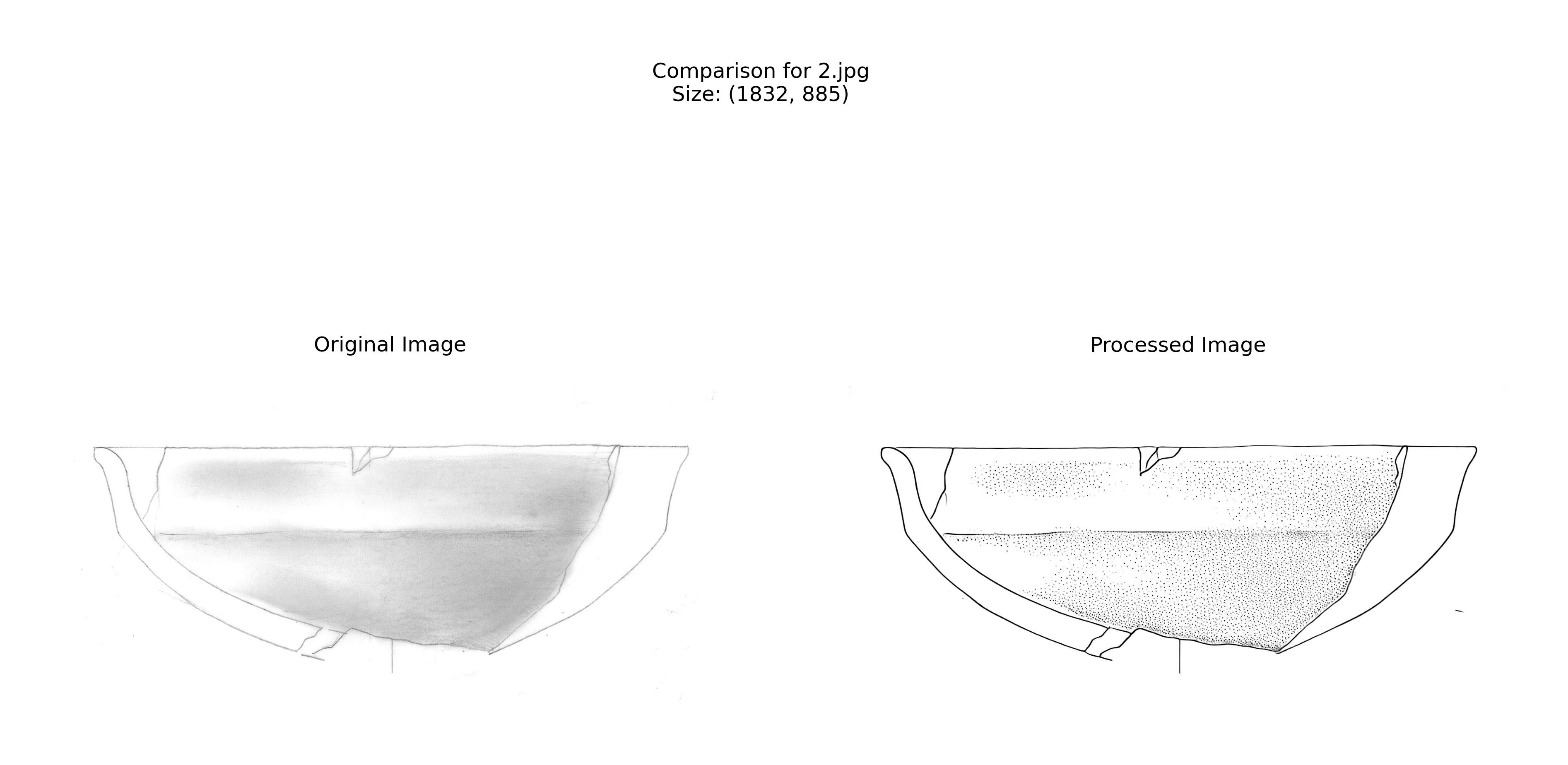
[Processing details...]

The comparison images (Figure 3) help us verify the quality of our results:

Figure 3: Side-by-side comparison showing the transformation from pencil drawing to inked version.

Best Practices and Troubleshooting

To get the best results from your processing:

1. Always start with diagnostics, even if you’re familiar with the model. Different collections might require slightly different parameters.
2. Pay attention to image resolution. The model works best with clear, well-scanned drawings. If your scans are too light or too dark, consider adjusting them before processing (Section 3).
3. Monitor the processing logs. If you see many failed conversions, it might indicate issues with your input images or parameters.
4. Review the comparison images carefully. They can help you spot any systematic issues that might need addressing.
5. Upscaling can help achieve a better result, especially when dealing with complex decorations. Upscaling factor is just for processing. The upscaling factor is for processing only. It doesn’t affect the output size.

Important

Remember that while this tool automates much of the inking process, it’s still important to review the results with an archaeological perspective. The model is a tool to assist, not replace, archaeological expertise.

Post-Processing Tools for Archaeological Drawings

Introduction

After generating inked versions of archaeological drawings, we often need to refine the results to meet some publication requirements or enhance the result. The post-processing module provides tools for image binarization, background removal, and stippling pattern enhancement. This guide will walk you through the main functions and best practices for using these tools.

Required Libraries

Let’s start by importing the necessary functions:

from postprocessing import (
    binarize_image,
    remove_white_background,
    process_image_binarize,
    binarize_folder_images,
    enhance_stippling,
    modify_stippling,
    control_stippling
)

Binarization and Background Removal

For many publication contexts, we want to remove the white background to create binary transparent images that can be easily integrated into figures:

# You can combine binarization and background removal in one step:
processed_image = process_image_binarize(
    image_path="path/to/image.jpg",
    binarize_threshold=127,
    white_threshold=250,
    save_path="output.png"  # Must use PNG to preserve transparency
)

Here the result:

Original ink

Binarized and background-clear image

Batch Processing

When working with multiple drawings, you can process an entire folder at once:

binarize_folder_images(
    input_folder="path/to/drawings",
    binarize_threshold=127,
    white_threshold=250
)

This creates a new folder with “_binarized” suffix containing processed images

Advanced Stippling Control

By using the post-processing module you can enhance and modify stippling patterns, check out this example!

Enhancing Stippling Patterns

First, we can isolate and enhance existing stippling patterns:

# Separate the main drawing from stippling patterns
processed_img, stippling_pattern = enhance_stippling(
    img=Image.open("drawing.png"),
    min_size=80,     # Minimum size of dots to preserve
    connectivity=2    # How dots connect to form patterns
)

The function returns two images:

• processed_img: Main drawing without small dots
• stippling_pattern: Isolated stippling pattern

Image without dotting

Isolated dotting

Modifying Stippling

Once we’ve isolated the stippling patterns, we can modify them in several ways:

modified_image = modify_stippling(
    processed_img=processed_img,
    stippling_pattern=stippling_pattern,
    operation='dilate',  # Options: 'dilate', 'fade', or 'both'
    intensity=0.5,      # Controls strength of dilation (0.0-1.0)
    opacity=1.0         # Controls darkness of stippling (0.0-1.0)
)

The operation parameter offers three different modification approaches:

• ‘dilate’: Makes dots larger while maintaining their density
• ‘fade’: Adjusts the opacity of dots without changing their size
• ‘both’: Combines dilation and opacity adjustments

Here a bunch of examples:

First, we increase the dots using the “dilate” option:

Secondly, we try to adjust the opacity using the fade option:

Finally, we combine the techniques:

Batch Stippling Control

For consistent stippling across multiple drawings:

control_stippling(
    input_folder="path/to/drawings",
    min_size=50,          # Size threshold for dot detection
    connectivity=2,        # How dots connect to each other
    operation='fade',      # Type of modification
    intensity=0.5,        # Strength of effect
    opacity=0.5           # Final opacity of stippling
)

This creates a new folder with “_dotting_modified” suffix containing the processed images.

Understanding the Parameters

When working with the stippling controls, it’s important to understand how different parameters affect the result:

• min_size: Controls which dots are considered part of stippling patterns versus actual drawing elements. Larger values preserve only larger dots.
• connectivity: Determines how dots are grouped together. Higher values (2 or 3) allow more diagonal connections.
• intensity: When dilating, controls how much dots expand. Values between 0.3-0.7 usually give the best results.
• opacity: Controls the final darkness of stippling patterns. Lower values create lighter shading.

Best Practices

1. Always work with high-resolution images to ensure clean binarization.
2. Start with conservative threshold values and adjust as needed.
3. Save intermediate results when working with stippling modifications.
4. Test your parameters on a small sample before processing entire collections.

Preprocessing Pipeline Documentation

Introduction to Image Preprocessing

Archaeological drawings often vary in their characteristics due to different artists, scanning conditions, and original materials. These variations can impact the performance of the model. This guide outlines the preprocessing pipeline that helps standardise images before they are processed by the model.

Import Required Libraries

from ink import process_folder, process_single_image
from preprocessing import DatasetAnalyzer, process_image_metrics, 
                visualize_metrics_change, process_folder_metrics

Understanding the Problem: Image Metric Variations

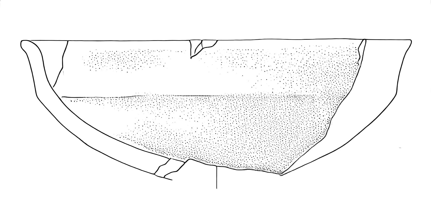
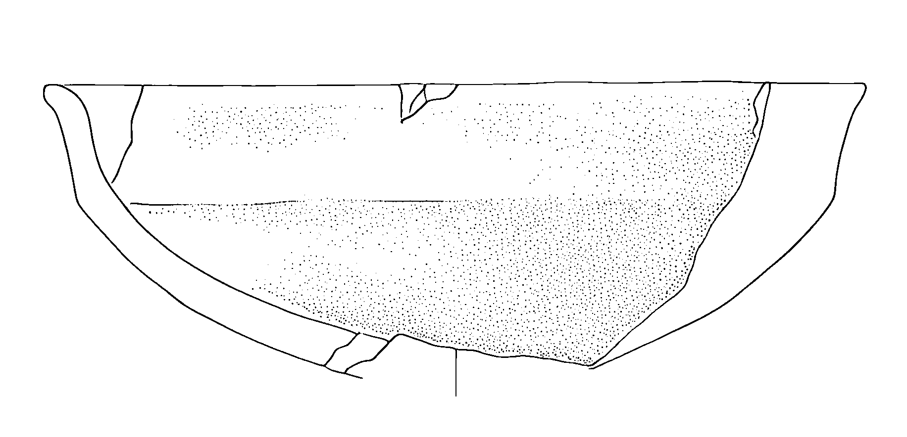
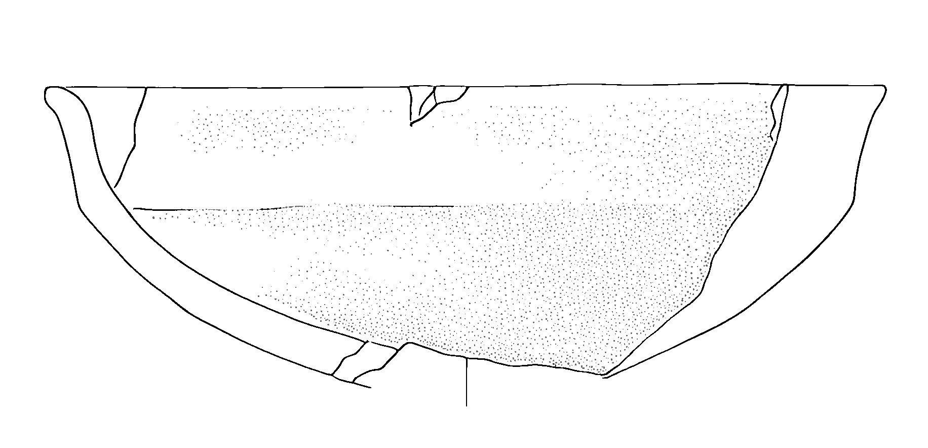
Let’s examine a specific case that illustrates why preprocessing is necessary. Consider the following high-contrast image (Figure 4).

Figure 4: An archaeological drawing with excessive contrast. The high contrast is evident in the black areas

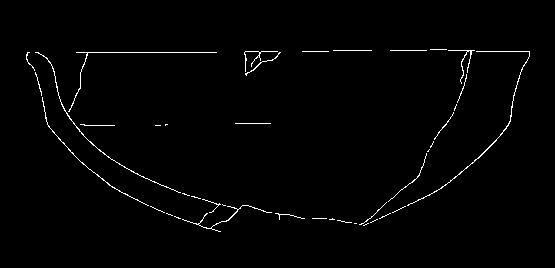
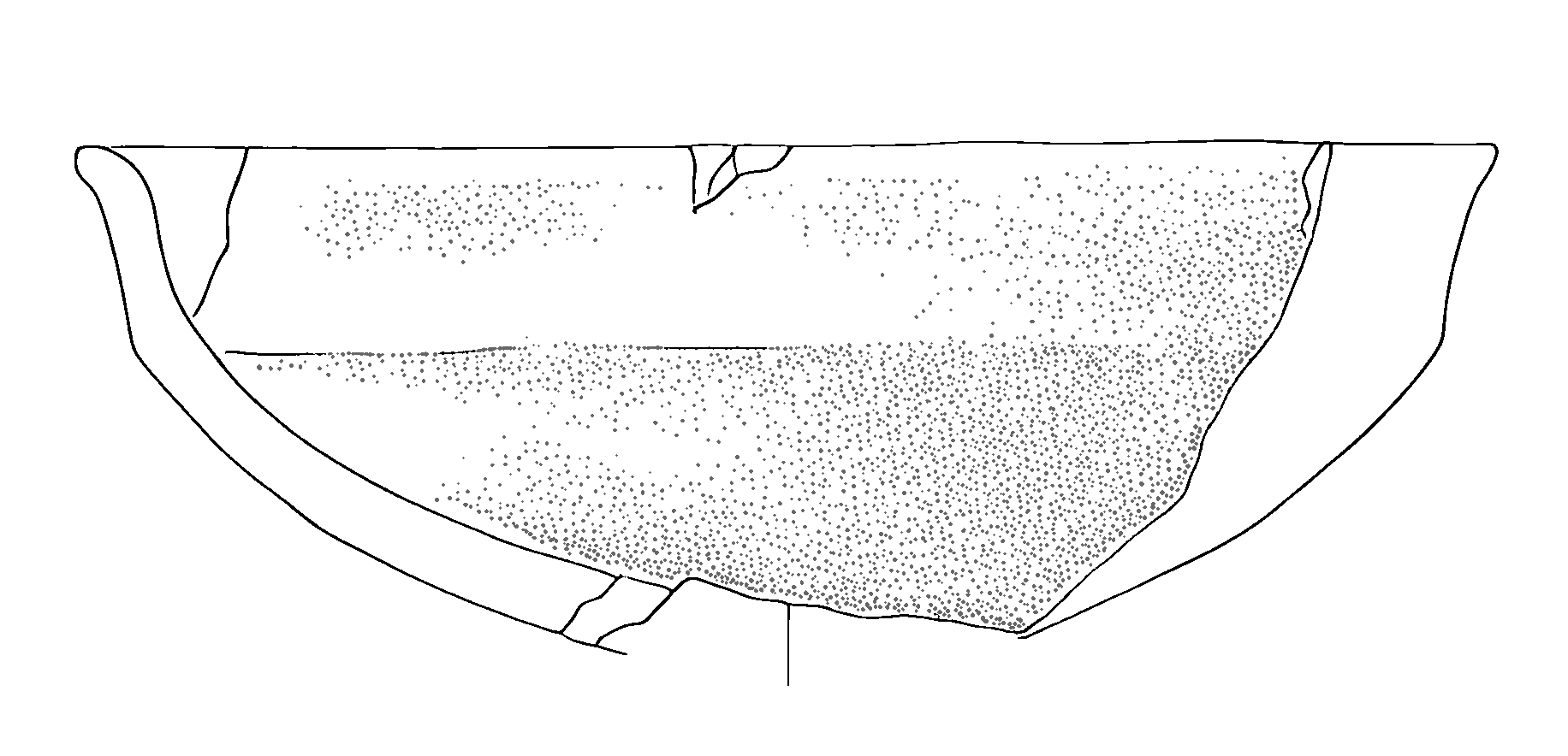
When we apply our model directly to this image without preprocessing, we get problematic results (Figure 5):

Figure 5: Direct model application showing artefacts. Note the missing dotting patterns and blue tiling artefacts in the bottom-right region.

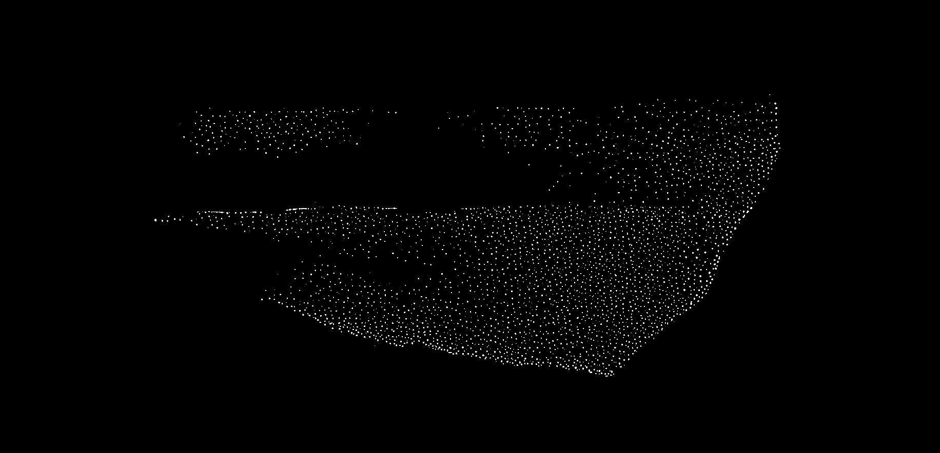
The output shows two significant issues:

1. Missing dot patterns in shaded areas
2. Unwanted blue tiling artefacts, particularly visible in the bottom-right section

These issues arise because the input image’s characteristics deviate significantly from the training dataset’s standard properties. Our preprocessing pipeline addresses this by analysing and adjusting key image metrics to align them with our training data distribution.

Image Metrics Analysis

The DatasetAnalyzer class calculates eight key metrics that characterise archaeological drawings:

1. Mean brightness: Overall lightness of the image
2. Standard deviation: Measure of tonal variation
3. Contrast ratio: Ratio between the brightest and darkest areas
4. Median: Middle intensity value
5. Dynamic range: Difference between the 99th and 1st percentile intensities
6. Entropy: Measure of information content
7. IQR (Interquartile Range): Spread of middle 50% of intensity values
8. Non-empty ratio: Proportion of pixels above background threshold

You can either analyse your own dataset to establish reference metrics or use our pre-computed metrics from the training dataset:

# Option 1: Analyse your own dataset
analyzer = DatasetAnalyzer()
model_stats = analyzer.analyze_dataset('PATH_TO_YOUR_DATASET')
analyzer.save_analysis('DATASET_RESULTS_PATH')

# Option 2: Use pre-computed metrics
analyzer = DatasetAnalyzer()
analyzer = analyzer.load_analysis('Montale_stats.npy')
model_stats = analyzer.distributions

The distribution of these metrics can be visualized:

analyzer.visualize_distributions_kde()

Figure 6: Figure 6: Distribution of image metrics from the training dataset. Each plot shows the distribution curve, actual data points, mean (red dashed line), median (blue dotted line), and ±2σ range (green shading).

Preprocessing Pipeline

The preprocessing pipeline adjusts images to match the statistical properties of the training dataset. Here’s how to process a single image:

original_image = 'PATH_TO_YOUR_IMAGE'
adjusted_image, adjusted_metrics = process_image_metrics(original_image, model_stats)

The pipeline performs these adjustments:

1. Contrast normalization based on the training set’s contrast ratio distribution
2. Dynamic range adjustment to match the target range
3. Brightness correction to align with the training set’s mean intensity

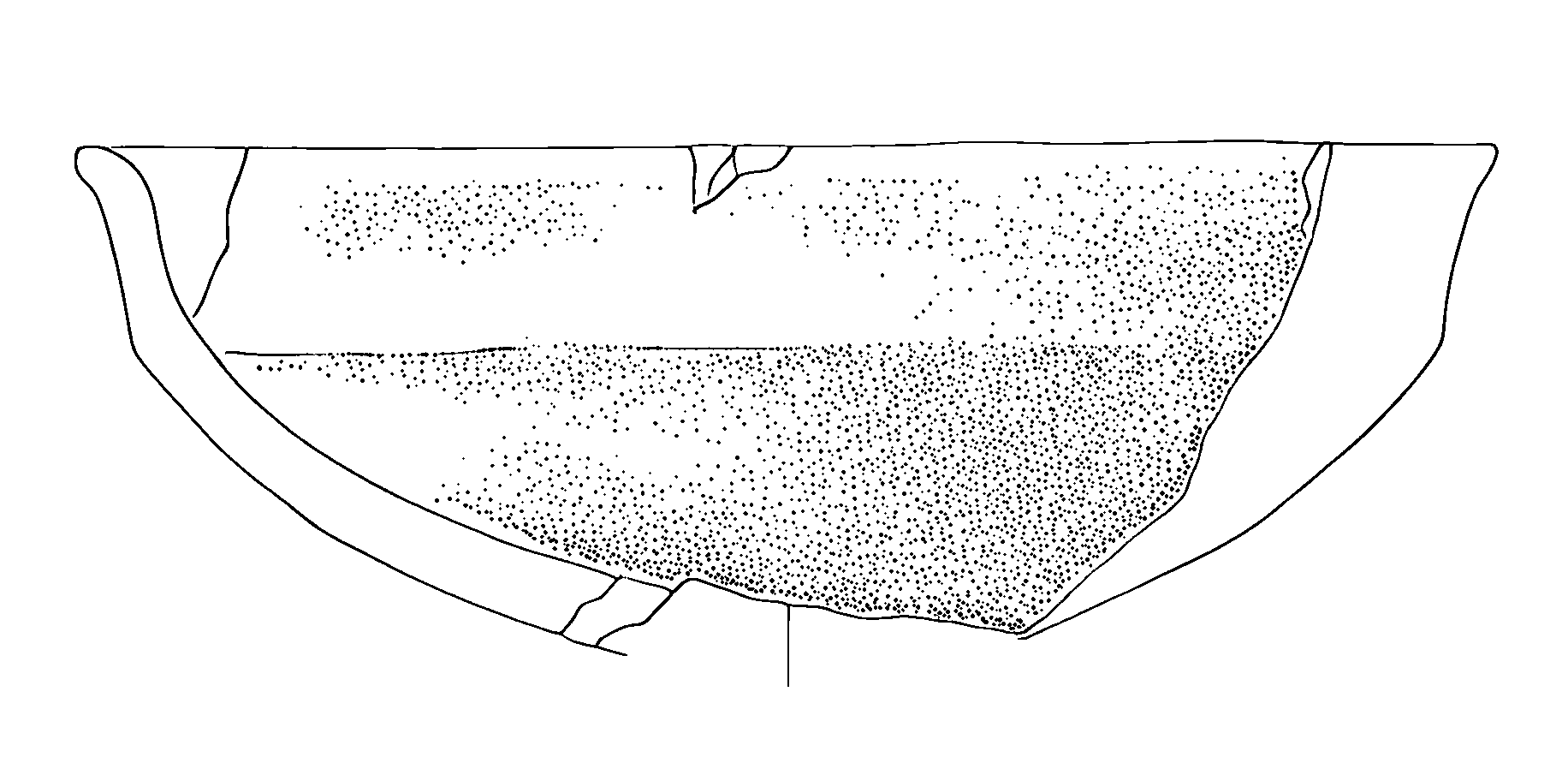
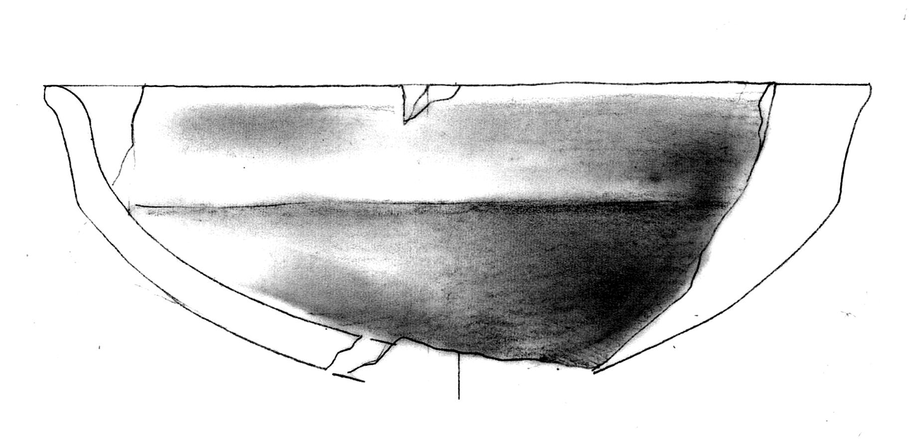
The adjusted image shows more balanced contrast and better preservation of details:

Figure 7: Figure 7: Preprocessed image showing normalized contrast and preserved details.

We can visualize how the preprocessing affected our image metrics:

Figure 8: Figure 8: Comparison of original (orange) and adjusted (teal) metrics against the training distribution.

Model Application

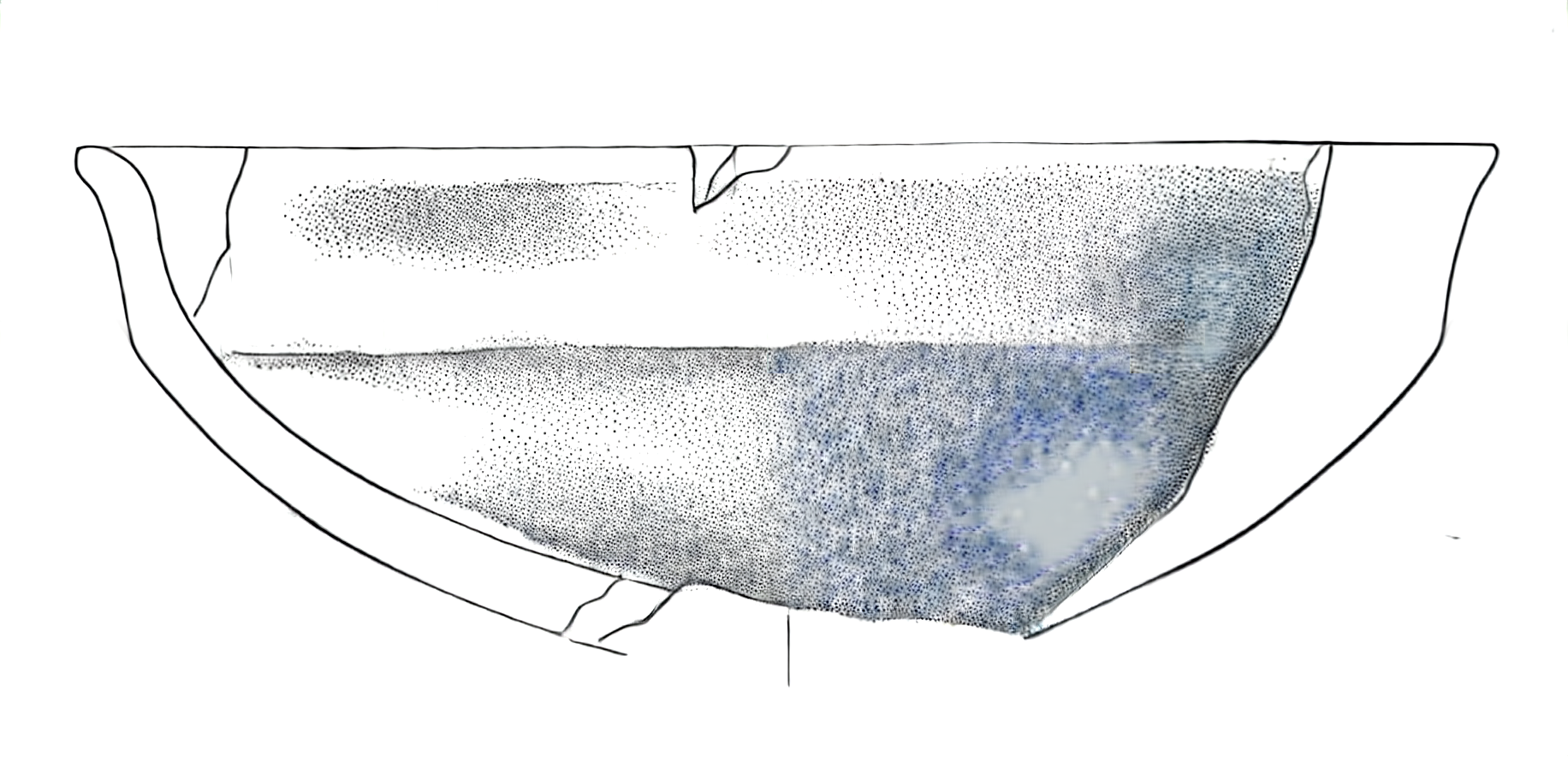
After preprocessing, the model produces significantly better results:

Figure 9: Figure 9: Model output after preprocessing, showing proper dotting patterns and no artifacts.

The improvements include:

• Consistent dotting patterns in shaded areas
• No colour artefacts or tiling effects
• Better preservation of fine details
• More natural transition between different tonal areas

I’ll add a section about batch processing to the documentation:

Batch Processing

While processing individual images is useful for testing and fine-tuning parameters, in archaeological practice we often need to process entire collections of drawings. The process_folder_metrics function automates this task by applying our preprocessing pipeline to all images in a directory.

Here’s how to use batch processing:

# Define the input folder containing your drawings
input_folder = "path/to/your/drawings"

# Process all images in the folder
process_folder_metrics(
    input_folder=input_folder,
    model_stats=model_stats,
    file_extensions=('.jpg', '.jpeg', '.png')  # Supported file formats
)

The function creates a new directory named input_folder_adjusted that contains all the processed images. During processing, it provides detailed feedback about each image:

📁 Found 25 images to process
==================================================

🔍 Analyzing: drawing_001.jpg
⚙️ Image Analysis:
└─ Contrast: 0.85x | Brightness adjustment needed
✨ Adjustments applied

Progress: 1/25
--------------------------------------------------

🔍 Analyzing: drawing_002.jpg
✅ Image metrics within normal ranges

Progress: 2/25
--------------------------------------------------

At the end of processing, you’ll receive a summary report:

📊 Processing Summary
==================================================
Total processed:  25
Images adjusted:  18
No adjustments:   7

💾 All images saved to: path/to/your/drawings_adjusted

This summary helps you understand how many images required adjustment, which can be useful for:

• Identifying systematic issues in your drawing or scanning process
• Planning future preprocessing strategies
• Documenting the processing pipeline for publication

The batch processing maintains all the benefits of individual processing while saving time and ensuring consistency across your entire dataset. All adjusted images will have metrics that align with your training data distribution, leading to better results when applying the model.

Note that each image still receives individual analysis and custom adjustments - the batch process doesn’t apply a one-size-fits-all transformation. Instead, it analyses each drawing’s specific characteristics and applies the precise adjustments needed to bring that particular image into alignment with your target metrics.

Guide to Fine-tuning PyPotteryInk Models

This guide walks you through the process of fine-tuning a PyPotteryInk model for your specific archaeological context.

Prerequisites

Before starting the fine-tuning process, ensure you have:

1. A GPU with at least 20GB VRAM for training
2. Python 3.10 or higher
3. A paired dataset of pencil drawings and their inked versions
4. Storage space for model checkpoints and training data

Environment Setup

1. First, clone the repository:

   git clone https://github.com/GaParmar/img2img-turbo.git

2. Install the required dependencies:

   pip install -r img2img-turbo/requirements.txt
   pip install git+https://github.com/openai/CLIP.git
   pip install wandb vision_aided_loss huggingface-hub==0.25.0

Dataset Preparation

1. To create a training dataset check out the original docs

2. Important considerations for dataset preparation:

   • Images should be paired (same filename in both folders)
   • Standard image formats (jpg, jpeg, png) are supported
   • Both pencil and inked versions should be aligned
   • Recommended resolution: at least 512x512 pixels

3. Data requirements:

   • Minimum recommended: 10-20 pairs for fine-tuning
   • Each drawing should be clean and well-scanned
   • Include variety in pottery types and decorations
   • Consistent drawing style across the dataset

Setting Up Fine-tuning

To fine-tune a pre-trained model (like “6h-MCG”), you’ll need to modify the base img2img-turbo repository. This enables the use of a pre-trained model as a starting point for your specialised training.

1. Prepare the Repository:
   • Navigate to your cloned img2img-turbo directory

   cd img2img-turbo

2. Replace Key Files:
   • Copy these files from the PyPotteryInk repository’s “fine-tuning” folder into the src folder:
     • pix2pix_turbo.py
     • train_pix2pix_turbo.py
   These modified files contain the necessary adaptations to support training from a pre-trained model.

Running Fine-tuning

1. Initialize Accelerate Environment:

   accelerate config

   This will guide you through setting up your training environment. Follow the prompts to configure for your GPU setup.

2. Start Training:

   accelerate launch src/train_pix2pix_turbo.py \
       --pretrained_model_name_or_path="6h-MCG.pkl" \
       --output_dir="YOUR_OUTPUT_DIR" \
       --dataset_folder="YOUR_INPUT_DATA" \
       --resolution=512 \
       --train_batch_size=2 \
       --enable_xformers_memory_efficient_attention \
       --viz_freq 25 \
       --track_val_fid \
       --report_to "wandb" \
       --tracker_project_name "YOUR_PROJECT_NAME"

   Key Parameters:

   • pretrained_model_name_or_path: Path to your pre-trained model (e.g., “6h-MCG.pkl”)
   • output_dir: Where to save training outputs and checkpoints
   • dataset_folder: Location of your training dataset
   • resolution: Image resolution (512 recommended)
   • train_batch_size: Number of images per training batch
   • viz_freq: How often to generate visualization samples
   • track_val_fid: Enable FID score tracking
   • tracker_project_name: Your Weights & Biases project name

   Note: Adjust the batch size based on your GPU memory. Start with 2 and increase if your GPU can handle it.

Important Considerations

• Ensure your pre-trained model file (e.g., “6h-MCG.pkl”) is in the correct location
• Monitor GPU memory usage during training
• Use Weights & Biases (wandb) to track training progress
• Check the output directory periodically for sample outputs
• Training time will vary based on your GPU and dataset size