Introduction

Archaeological drawing digitisation represents a crucial step in preserving and sharing our cultural heritage. While traditionally done by hand, modern computational methods can help streamline this process while maintaining the high standards required for archaeological documentation. This guide walks you through using the ink module, a specialised tool designed for converting pencil drawings of archaeological artefacts into publication-ready inked versions.

Setting Up Your Environment

Let’s begin by importing the necessary functions from the toolset:

from ink import process_folder, run_diagnostics

These two functions serve as the foundation of our processing pipeline. The run_diagnostics function helps us understand how our images will interact with the model, while process_folder handles the actual conversion process.

Think of run_diagnostics as our planning phase and process_folder as our execution phase.

Understanding the Diagnostic Process

Before processing an entire collection of drawings, we need to understand how our specific drawings will interact with the model.

First, let’s set up our working directory:

my_path = "Montale_example"

Now we can run our diagnostic analysis:

run_diagnostics(
    input_folder=my_path,           # Where your drawings are stored
    model_path="6h-MCG.pkl",        # The trained model file
    num_sample_images=1,            # How many test images to analyze
    contrast_values=[0.5, 0.75, 1, 1.5, 2, 3],  # Different contrast levels to test
)

Let’s understand each parameter in detail:

input_folder: This is where your pencil drawings are stored. The function will randomly select images from this folder for analysis.
model_path: Points to your trained model file. This model contains the learned patterns for converting pencil drawings to inked versions.
num_sample_images: Controls how many images to analyse. For a small collection, 1-2 images might suffice, but for larger collections with varying drawing styles, you might want to test more.
contrast_values: These values help us understand how different contrast levels affect the model’s output. Think of this like adjusting the pressure of your pen when inking - too light (low contrast) might lose details, while too heavy (high contrast) might create unwanted artefacts.

The diagnostic process creates a structured output that helps us understand how our images will be processed:

diagnostic/
├── contrast_analysis_{progressive_number}.png  # Shows how contrast affects results
├── patches_{progressive_number}.png            # Shows how images will be divided
└── summary_{progressive_number}.txt            # Contains detailed analysis

Let’s examine the patch division output (Figure 1):

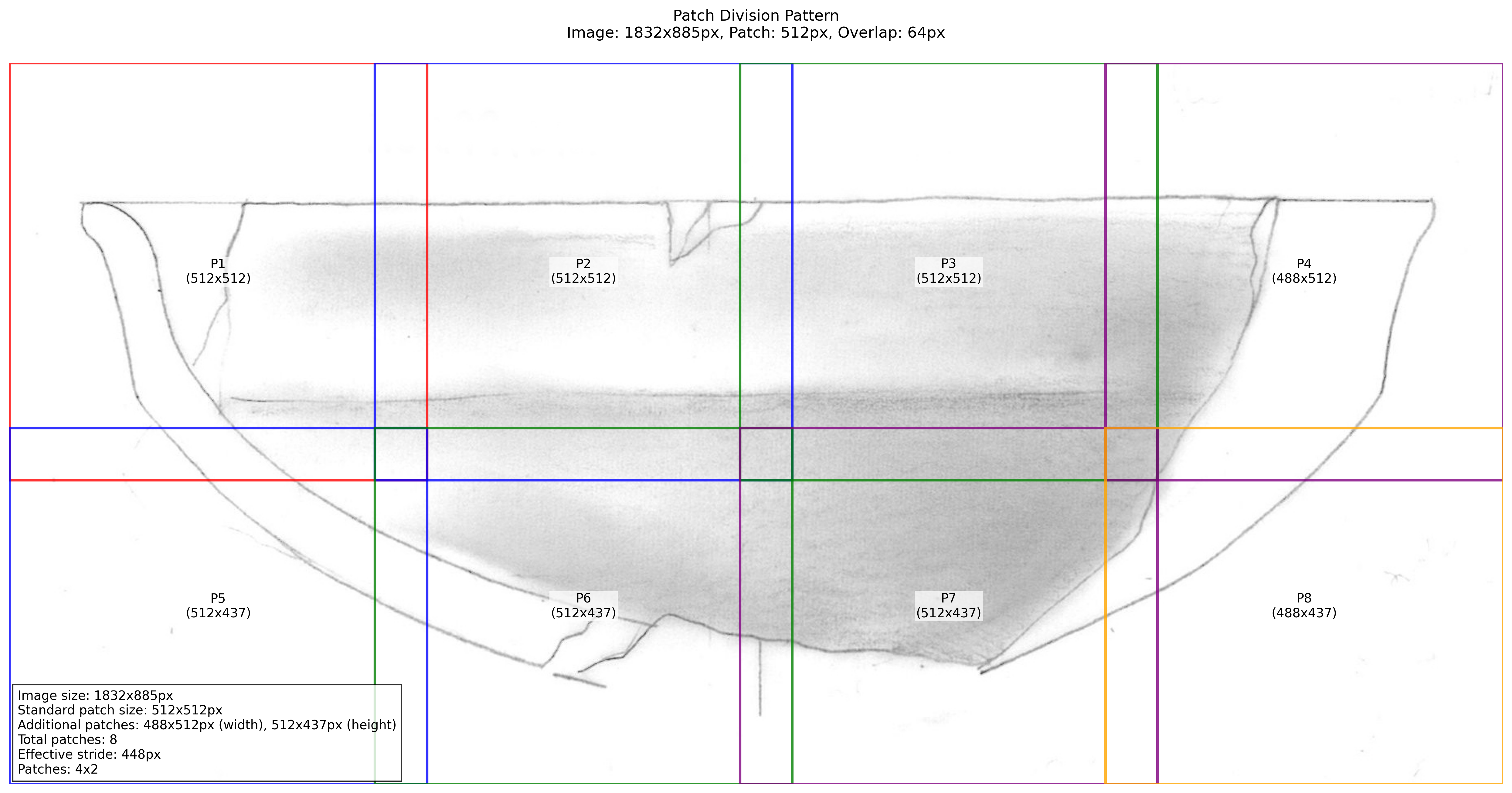
Figure 1: This visualization shows how your image will be processed in smaller chunks. The green lines indicate patch boundaries, while yellow areas show where patches overlap to ensure smooth transitions.

The patch division is crucial because it shows us how the model will break down larger images into manageable pieces. The overlap between patches helps prevent visible seams in the final output.

Next, let’s look at the contrast analysis (Figure 2):

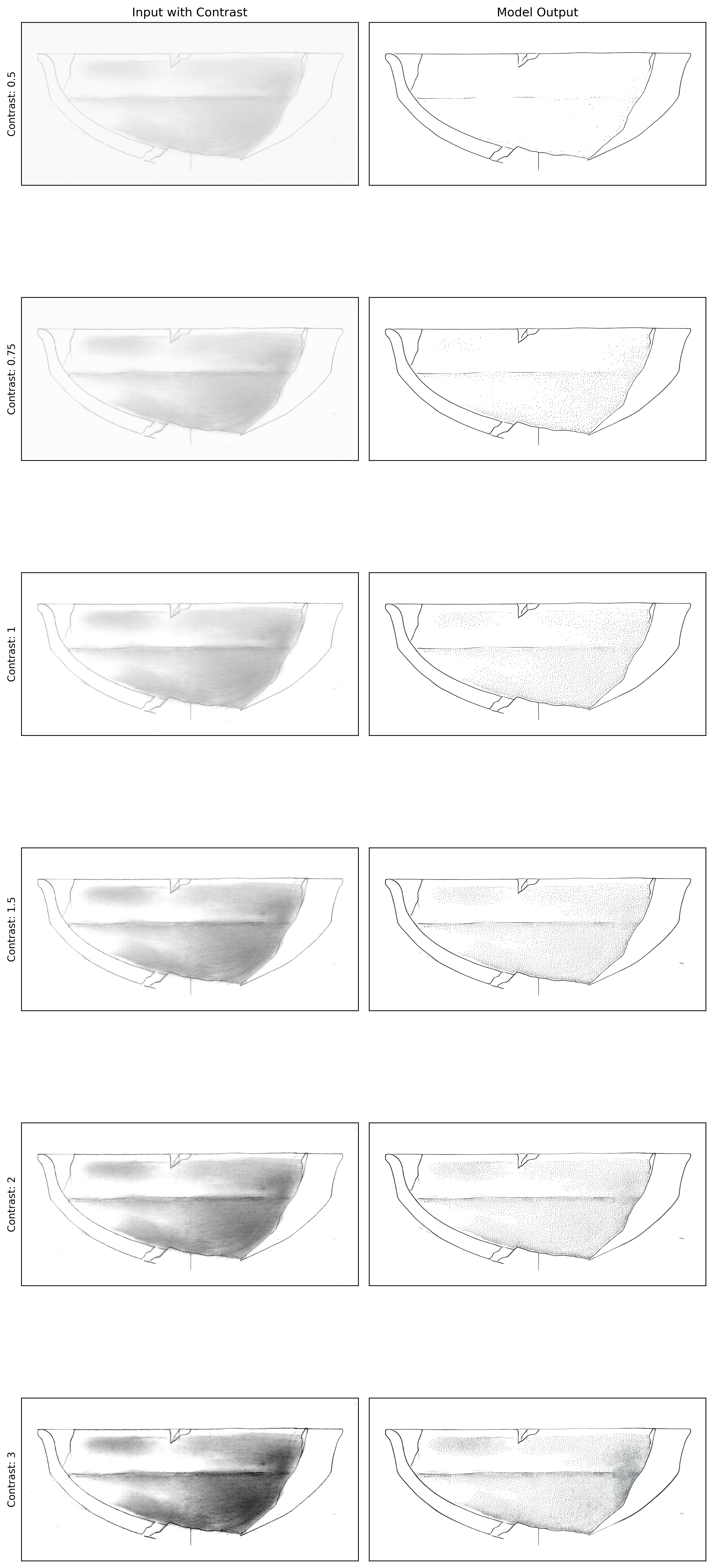
Figure 2: This analysis shows how different contrast values affect the model’s output. Notice how extreme values can either lose detail (too low) or create artefacts (too high).

This visualization is particularly important because it helps us find the sweet spot for contrast enhancement. Looking at the results:

A contrast value of 0.5 is too low, causing loss of fine details
A contrast value of 3.0 is too high, introducing unwanted artefacts
Values between 1.0 and 1.5 seem to produce the most balanced results

Processing Your Collection

After understanding how our images interact with the model through diagnostics, we can proceed with processing our entire collection:

process_folder(
    input_folder=my_path,
    model_path="6h-MCG.pkl",
    contrast_scale=1.25,            # Chosen based on diagnostic results
    output_dir="Montale_processed", # We define an output folder
    use_fp16=True,                  # Enables faster processing
    upscale=1                       # Upscale the image (1: no upscaling)
)

The processing creates an organized output structure that helps us track and validate our results:

Montale_processed/
├── comparisons/                # Before/after comparisons
│   ├── comparison_{image_name}.jpg
├── logs/                       # Detailed processing records
│   └── processing_log_{timestamp}.txt
├── {image_name}.jpg           # Final processed images

The log files contain valuable information about the processing:

Processing started at: 2024-12-30 13:26:26.607305
Configuration:
- Input folder: Montale_example
- Output directory: Montale_processed
- Model path: model_601.pkl
- FP16 mode: True
- Patch size: 512px
- Overlap: 64px
- Contrast scale: 1.25
- Prompt: make it ready for publication

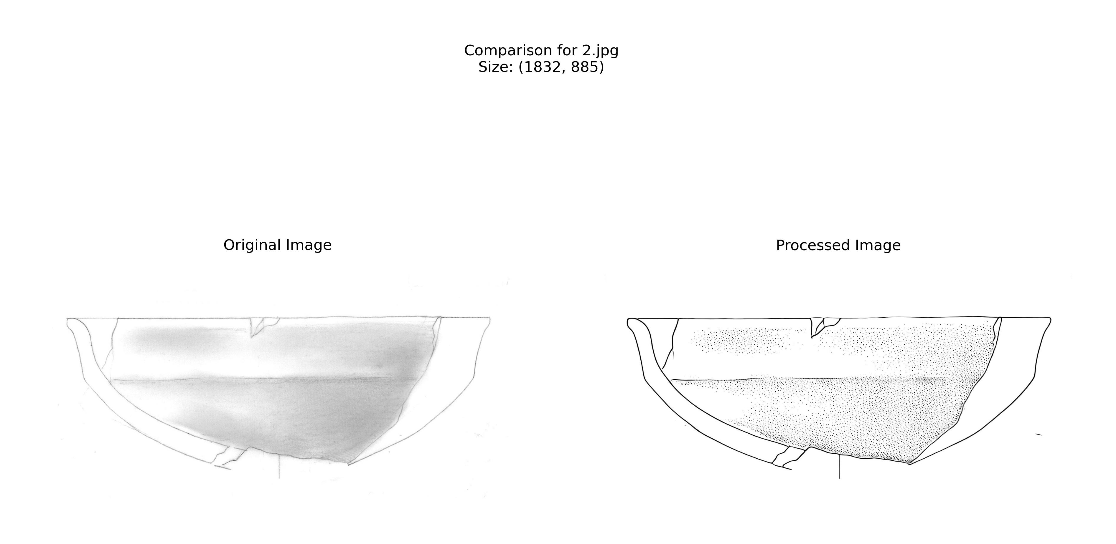
[Processing details...]

The comparison images (Figure 3) help us verify the quality of our results:

Figure 3: Side-by-side comparison showing the transformation from pencil drawing to inked version. Notice how the model maintains detail while creating clean, publication-ready lines.

Best Practices and Troubleshooting

To get the best results from your processing:

Always start with diagnostics, even if you’re familiar with the model. Different collections might require slightly different parameters.
Pay attention to image resolution. The model works best with clear, well-scanned drawings. If your scans are too light or too dark, consider adjusting them before processing (see preprocessing).
Monitor the processing logs. If you see many failed conversions, it might indicate issues with your input images or parameters.
Review the comparison images carefully. They can help you spot any systematic issues that might need addressing.
Upscaling can help achieve a better result, especially when dealing with complex decorations. Upscaling factor is just for processing. The upscaling factor is for processing only. It doesn’t affect the output size.

Important

Remember that while this tool automates much of the inking process, it’s still important to review the results with an archaeological perspective. The model is a tool to assist, not replace, archaeological expertise.